Deterministic Motor Control on FPGA: A Model-Based Approach
Deterministic Motor Control on FPGA: A Model-Based Approach
In motor control, being fast on average is not the goal. What matters is that the controller reads the sensor, computes and updates the output in the same time, every single cycle. A loop that is quick most of the time but occasionally late does not just lose performance; it loses phase margin, and with it stability.
This is where FPGAs earn their place. Not because they are always faster than a microcontroller, but because a control loop built in programmable logic is a fixed circuit: it takes the same number of clock cycles every time, regardless of what else the system is doing.
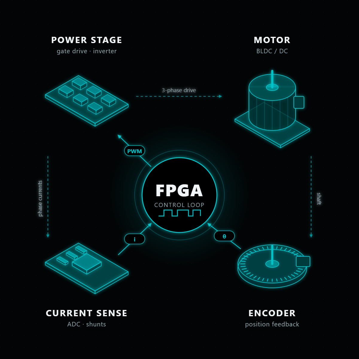
This article looks at motor control from that timing angle: how latency eats into stability, how high-rate loops and estimators fit on an FPGA, why the feedback path deserves as much attention as the controller, and how a model-based flow from Simulink to verified HDL makes the whole thing practical.
Latency Is a Phase Problem
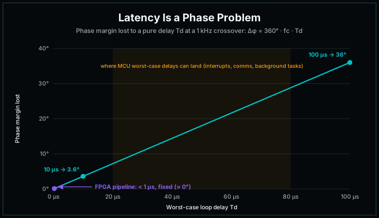
Every delay in a control loop removes phase margin. A pure time delay Td costs 360° · fc · Td of phase at the crossover frequency fc (ω·Td in radians), and it does so without changing the gain at all.
The numbers make the point. For a loop with a 1 kHz crossover frequency:
- A 10 µs delay costs about 3.6° of phase margin.
- A 100 µs delay costs about 36°.
The second case can turn a comfortably stable loop into one that rings or oscillates. And the delay that matters is not the average one. It is the worst case.
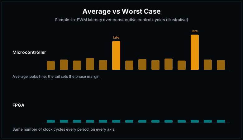
On a microcontroller, the time from sensor sample to PWM update is the sum of interrupt latency, computation time and whatever else the processor is handling: communication stacks, other interrupts, background tasks. The average can look fine while the worst case hides in the tail.
On an FPGA, the same computation is a pipeline. A PI controller running at 100 MHz finishes in a handful of clock cycles, tens to hundreds of nanoseconds, and it finishes in exactly the same number of cycles every time. The gap between average and worst-case latency is essentially zero, and adding a second or third axis does not change it, because each axis runs on its own hardware in parallel.
Higher Loop Rates, Richer Controllers
Once latency is small and fixed, the next lever is loop rate. A faster loop sees disturbances sooner, allows a higher bandwidth, and pushes sampling-related artefacts further away from the frequencies you care about. Sampling itself adds roughly half a sample period of delay, so a 10 kHz loop loses about 18° at a 1 kHz crossover before any computation is counted.
FPGAs handle high loop rates comfortably because the cost of a computation does not grow with how often you run it. A few examples of what becomes practical:
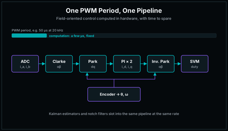
- Current loops in the tens of kHz. Field-oriented control needs current loops that run every PWM period. On an FPGA, Clarke and Park transforms, PI controllers and space-vector modulation all fit within one period, with time to spare.
- State estimators such as Kalman filters. A Kalman filter is mostly matrix multiplications and additions, exactly what DSP slices are built for. Running an estimator at the same rate as the control loop, rather than a slower background rate, improves the quality of the states the controller uses.
- Notch filters and resonance suppression. Mechanical resonances in gimbals, lens mechanisms and actuators can be attenuated with filters that run inside the loop without adding meaningful delay.
- Multi-axis control. In line-of-sight stabilisation, several axes must be controlled together. On an FPGA each axis gets its own pipeline, so the loop timing of one axis never depends on another.
The Feedback Path Sets the Limit
A controller can only be as good as the measurement it receives. In practice, the feedback path is often where motor control performance is won or lost.
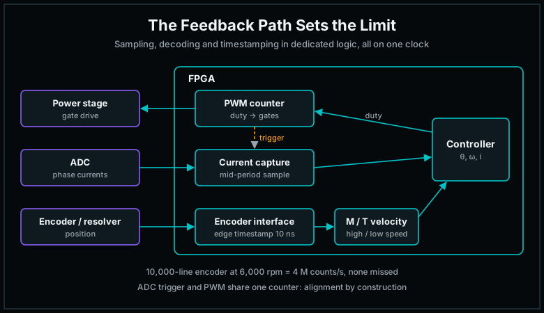
Encoder reading. A quadrature encoder with 10,000 lines gives 40,000 counts per revolution after 4× decoding. At 6,000 rpm, that is 4 million counts per second. The decoder must count every edge, filter glitches from noisy cables, and do it without ever missing a transition. In programmable logic, this is a small, dedicated circuit that runs independently of everything else.
Absolute encoders and resolvers. Interfaces such as BiSS-C, EnDat and SSI, or resolver-to-digital conversion, have strict timing on clock and data lines. Implementing them in the FPGA gives deterministic sampling and keeps the protocol timing out of software.
Velocity estimation. Speed is rarely measured directly; it is estimated from position. At high speed, counting pulses over a fixed period (the M method) works well. At low speed, there are too few pulses per period, and measuring the time between edges (the T method) gives a much better estimate. With a 100 MHz clock, the FPGA can timestamp each edge with 10 ns resolution, which makes accurate low-speed velocity estimation possible without extra hardware.
Sampling synchronisation. Current measurements should be taken in the middle of the PWM period, away from switching noise. In an FPGA, the ADC trigger is generated from the same counter that drives the PWM, so the timing relationship is guaranteed by construction, not by careful software scheduling.
A Model-Based Flow: From Simulink to Verified HDL
Writing control algorithms directly in HDL works, but it is slow to change. Every time a gain is retuned or a filter is redesigned, the code has to be rewritten and re-verified. A model-based flow keeps the algorithm in one place and generates the hardware from it.
The flow we use looks like this:
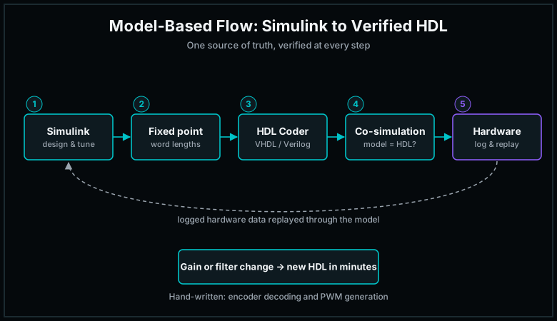
- Design the controller in Simulink. The control engineer designs the loop, the pre-filter and the estimator in the environment they already use, and tunes them against a plant model.
- Move to fixed point. Floating point in an FPGA costs logic, power and throughput, so the model is converted to fixed-point arithmetic. This is where most of the engineering judgement sits: too little resolution and the controller degrades through quantisation; too much and resources are wasted. Word and fraction lengths are chosen from simulation, not guessed.
- Generate HDL. HDL Coder turns the fixed-point model into VHDL or Verilog. Interfaces that are timing-critical, such as encoder decoding and PWM generation, are usually written by hand and kept separate.
- Co-simulate. The Simulink model and the generated HDL are simulated side by side, with the same input stimulus driving both, and their outputs are compared. Only when they match does the generated code go to synthesis.
- Verify on hardware. Real signals, such as target position, measured position, filter output and controller output, are logged from the running system and replayed through the model. When the logged hardware behaviour matches the simulation, the implementation is verified against the design, not just against a test case.
The biggest benefit is change. If the gains, the filter cut-off or the filter order change, new HDL is generated from the updated model in minutes, and the same co-simulation setup verifies it again.
From My Earlier Work: A Model-Based Position Controller
I first applied this flow in 2017, together with a colleague, on a DC motor position controller for an electro-optical system. The controller combined a first-order low-pass pre-filter, which softens step commands and reduces overshoot, with a discrete PI controller. Both were designed in Simulink, converted to fixed point, generated as VHDL with HDL Coder, and co-simulated against a gate-level HDL simulator. Encoder reading and PWM generation were written by hand.
The results on hardware:
| Metric | Result |
|---|---|
| Control loop rate | 10 kHz |
| Settling time | ~0.9 s |
| Steady-state error | 1 encoder step |
| Operating temperature | −32 °C to +55 °C, same precision |
The filter and controller together used 167 flip-flops, 411 LUTs and 11 DSP blocks on a low-cost FPGA. In other words, the control algorithm itself used only a small fraction of the device, leaving almost all of it for the rest of the system.
Logged hardware data, replayed through the Simulink model, matched the simulation closely. The small differences that remained came from the data logging rate (1 kHz, versus the 10 kHz controller rate) and from the initial state of the pre-filter in simulation, not from the implementation.
I presented this work at MATLAB EXPO Türkiye 2018, and it was published in FIGES’ Advanced Engineering and R&D Technologies magazine (2018/3, Issue 19).
Model-Based Design in DO-254 Projects
In airborne programmes, FPGA designs are developed under DO-254, and the same model-based flow fits naturally into that process when it is planned for from the start.
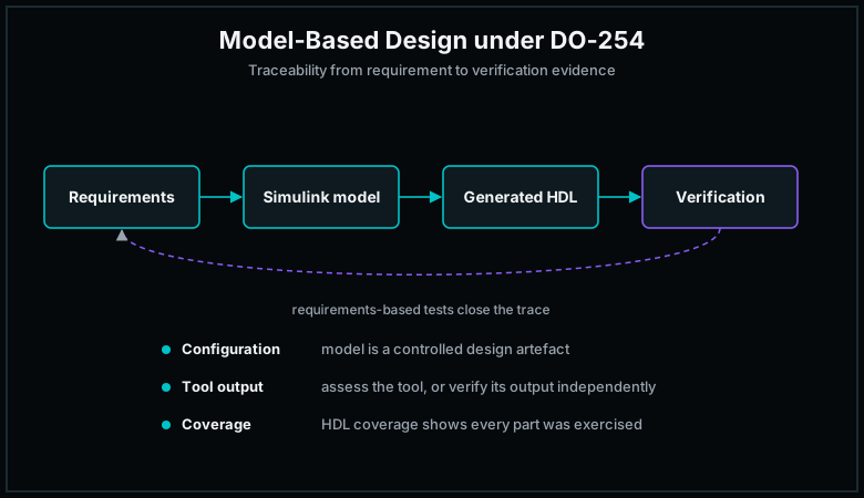
- Traceability. Requirements trace to the model, the model to the generated HDL, and the HDL to verification results. The model becomes a design artefact under configuration management, not a throwaway prototype.
- Treating generated code as a design output. Code generated by a tool is not trusted by default. Either the tool is assessed and qualified, or its output is independently verified. Co-simulation against the model, together with requirements-based simulation, provides that independent verification evidence.
- Verification depth. For higher design assurance levels, requirements-based testing is complemented by additional methods, such as coverage analysis of the HDL, to show that every part of the design has been exercised.
At RunX we run DO-254 projects, and we have started bringing UVM-based verification into our IP development flow, so that the same structured, coverage-driven verification applies to our cores as well as to project designs.
When Is an FPGA the Wrong Choice?
Not every motor needs an FPGA. For a single axis at moderate speed, with a standard encoder and relaxed bandwidth requirements, a modern microcontroller with dedicated motor-control peripherals is often cheaper and simpler.
An FPGA becomes the right choice when one or more of these apply:
- The loop needs high bandwidth, so delay and jitter directly limit performance.
- Several axes must be controlled together with guaranteed timing.
- The feedback path uses demanding interfaces, high count rates or precise edge timestamping.
- An FPGA is already in the system for video, sensor or data processing, so the controller can share it.
- The application requires long product life, radiation tolerance or design assurance under DO-254.
A Practical Checklist
- Budget phase, not just time. Convert your worst-case loop delay into phase margin at the crossover frequency.
- Design for the worst case. Measure the maximum sample-to-output delay over a long run, not the average.
- Treat the feedback path as part of the controller. Encoder decoding, velocity estimation and sampling synchronisation set the ceiling on performance.
- Choose fixed-point formats from simulation. Check quantisation effects against the closed-loop response before generating HDL.
- Co-simulate before you synthesise. The generated HDL must match the model for the same stimulus.
- Close the loop on verification. Log hardware signals and replay them through the model to confirm the implementation.
Conclusion
Deterministic motor control is not about squeezing a few more microseconds out of a processor. It is about building a control loop whose timing is fixed by design: the same latency in every cycle, on every axis, under every load.
FPGAs make that possible, and a model-based flow makes it practical. The controller is designed and tuned where control engineers work, generated as hardware, and verified against the model at every step, from co-simulation to logged data from the real system.
If you are working on a motor control, stabilisation or actuator system that needs deterministic timing, we would be glad to talk.