Image Signal Processing on FPGAs: Pipelines and Noise Reduction
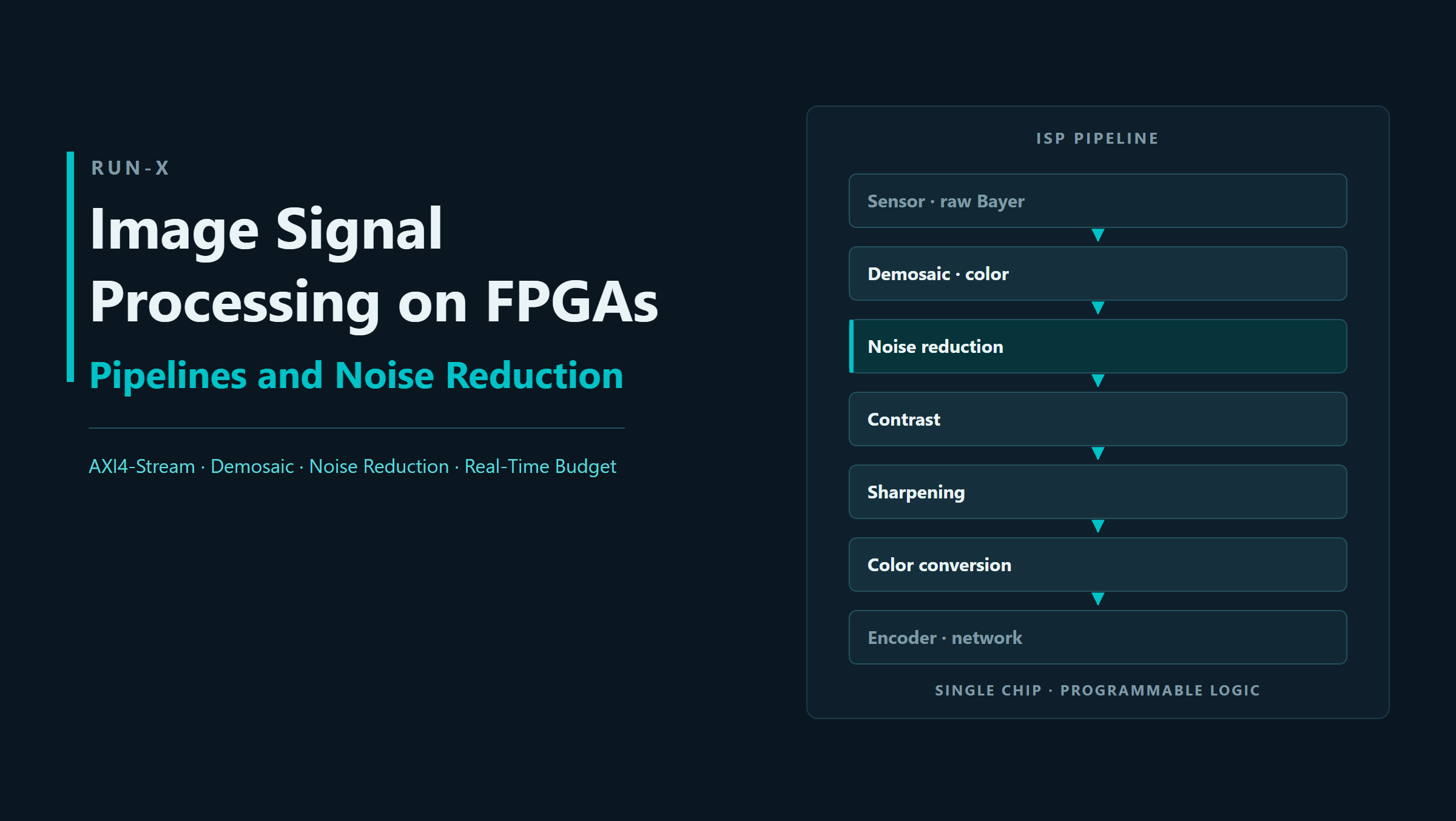
In a camera system, what the sensor sees and what you see on the screen are not the same thing. The data leaving the sensor is raw, flat, colorless and noisy. The structure that closes the gap between the two is the ISP, the image signal processing pipeline.
On desktop and mobile platforms this pipeline usually arrives as a finished block and you only tune its parameters. In embedded imaging systems you build the pipeline yourself. You decide which blocks exist, what order they sit in, and how many clock cycles each of them is allowed to take.
Drawing on the imaging pipelines we have built on FPGA SoC platforms, this article covers three things: which blocks make up the pipeline, why their order changes the result so much, and how noise reduction is designed so that it runs in real time.
What Does an ISP Pipeline Fix?
Raw sensor data is not something you can display directly. Some pixels are dead, the black level does not sit at zero, each pixel carries only one color channel, white does not look white, and noise is everywhere. The ISP pipeline closes each of these gaps with a separate block.
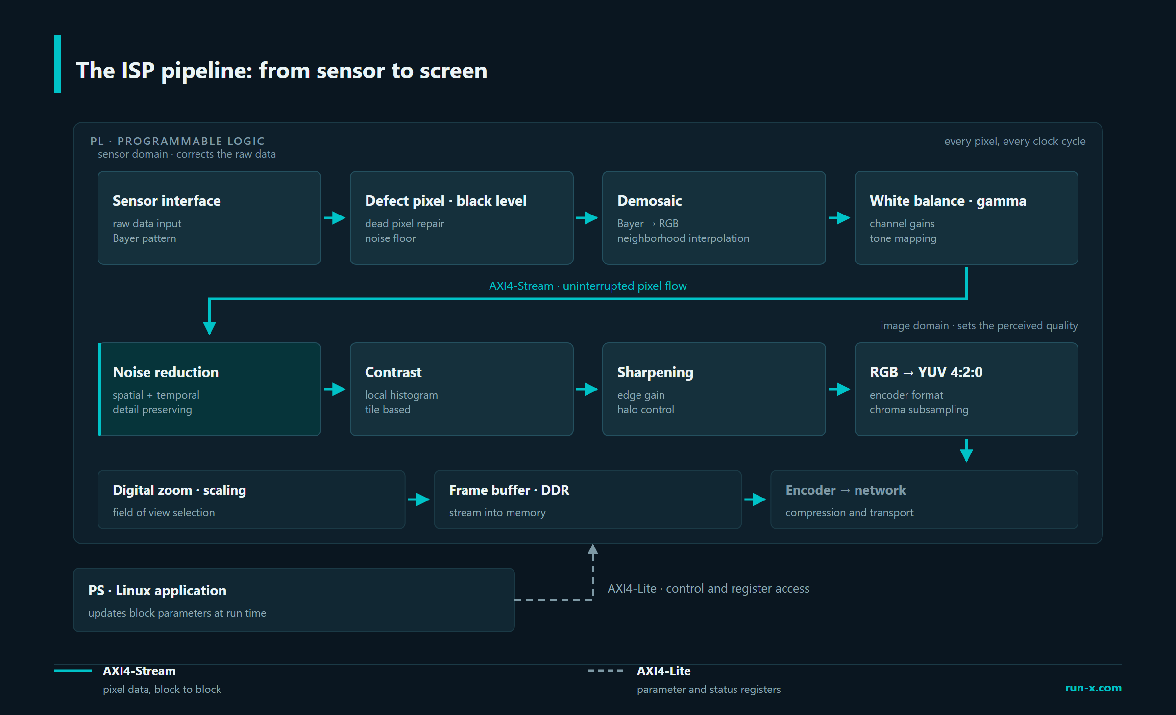
The first half of the pipeline works in the sensor domain and corrects the raw data: defect pixel repair, black level subtraction, demosaic, white balance and gamma. The second half works in the image domain and sets the perceived quality: noise reduction, contrast, sharpening, and conversion into the color format the encoder expects.
| Block | What it does | Why in programmable logic? |
|---|---|---|
| Defect pixel, black level | Removes fixed, sensor specific errors | Runs for every pixel, with fixed latency |
| Demosaic | Turns the Bayer pattern into a full color image | Needs a neighborhood window and line buffers |
| White balance, gamma | Color and tone mapping | Simple but per pixel; must not stall the stream |
| Noise reduction | Suppresses noise while preserving signal | The most expensive block; parallelism pays off here |
| Contrast | Local histogram equalization | Tile based, carries state across the frame |
| Sharpening | Edge gain | Amplifies noise too, so its position is critical |
| RGB to YUV 4:2:0 | The encoder input format | The last step on the way to the encoder |
We connect the blocks with AXI4-Stream. That interface has no concept of an address; data flows continuously, and when the receiver is not ready it slows the stream down through the tready signal. No block in the pipeline gets to say “I will deal with it later”. A pixel is processed when it arrives and leaves at the rate it arrived.
Parameters, on the other hand, are updated from the application on the processor side over AXI4-Lite. While the image keeps flowing, the user can change threshold and gain values. This separation is what the FPGA SoC architecture contributes most to image processing: the data path lives in programmable logic, the decisions and the control live on the processor.
Why Does the Order Matter So Much?
Arrange the same set of blocks in a different order and you get a very different image. The clearest example is the order of contrast and noise reduction.

Local contrast blocks amplify small brightness differences in flat regions. The trouble is that this is exactly what noise is: small brightness differences in flat regions. Apply contrast first and you lift the noise along with everything else. Sharpening then amplifies it once more. The filter you placed at the end of the pipeline is no longer facing noise but texture that used to be noise, and detail is lost in the process.
Put noise reduction first and the contrast block lifts signal instead of noise.
Sharpening carries a similar trade-off. As you raise the edge gain, sharpness increases up to a point and then saturates, while halo keeps growing. This is why the gain belongs at the very end of the pipeline and has to be set by measurement rather than by eye.
The working rule is simple: suppress noise before it enters the chain, and apply gain last.
Where Does the Noise Come From?
Image noise does not have a single source. Photon noise comes from physics and no sensor swap will remove it; it grows in relative terms as the signal gets weaker. Read noise comes from the electronic chain itself. Fixed pattern noise arises from small gain and offset differences between pixels, and it stays in the same place from frame to frame.
That distinction is useful in practice. Because fixed pattern noise is identical across frames, it can be corrected by calibration. Photon and read noise change randomly from frame to frame, and the only way to reduce them is to filter.
In low light all of it gets harder at once: the signal drops, the noise stays where it is, and the signal to noise ratio falls. Raising the gain is not a solution on its own, because it amplifies both.
Spatial or Temporal?
Because noise is random, averaging reduces it. The question is where you take the average from: neighboring pixels in the same frame, or the same pixel in earlier frames?
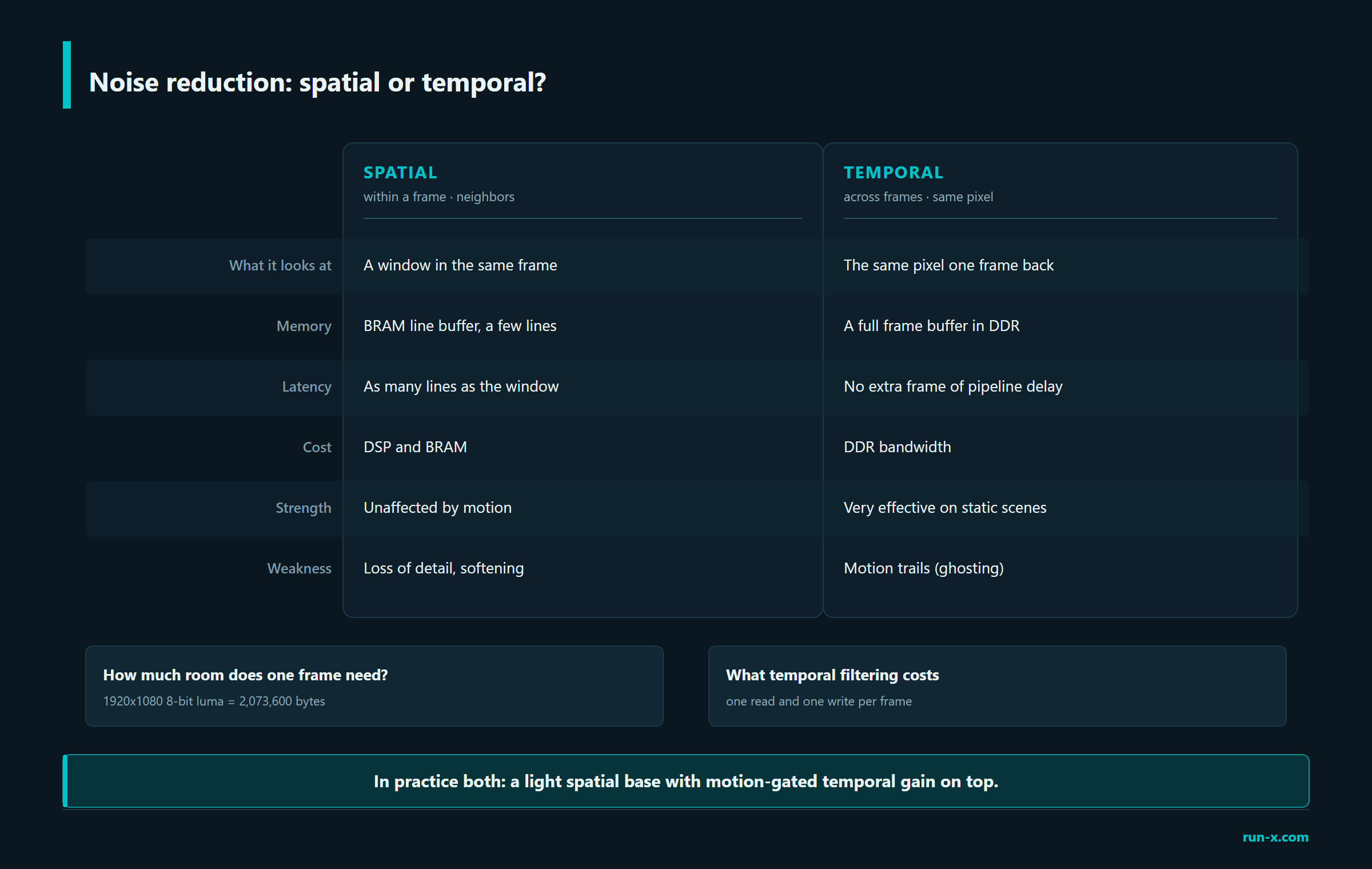
A spatial filter stays inside one frame. It uses neighboring pixels, needs a line buffer a few lines deep in BRAM, and is completely unaffected by motion. In return it averages the detail as well: it softens real texture along with the noise.
A temporal filter looks at the previous frame. It averages the values of the same pixel over time. When the scene is static the result is very strong, because real detail stays constant across frames while noise changes. But when the scene moves, that pixel no longer shows the same object, and averaging leaves a trail.
The costs differ too. A spatial filter spends DSP and BRAM. A temporal filter needs a full frame buffer; for 1920x1080 8-bit luma that is 2,073,600 bytes per frame, and every frame means one read and one write.
In practice the two are used together: a light spatial base with motion-gated temporal gain on top.
How to Build the Temporal Filter
The temporal filter raises exactly one difficult question: where does the previous frame come from?
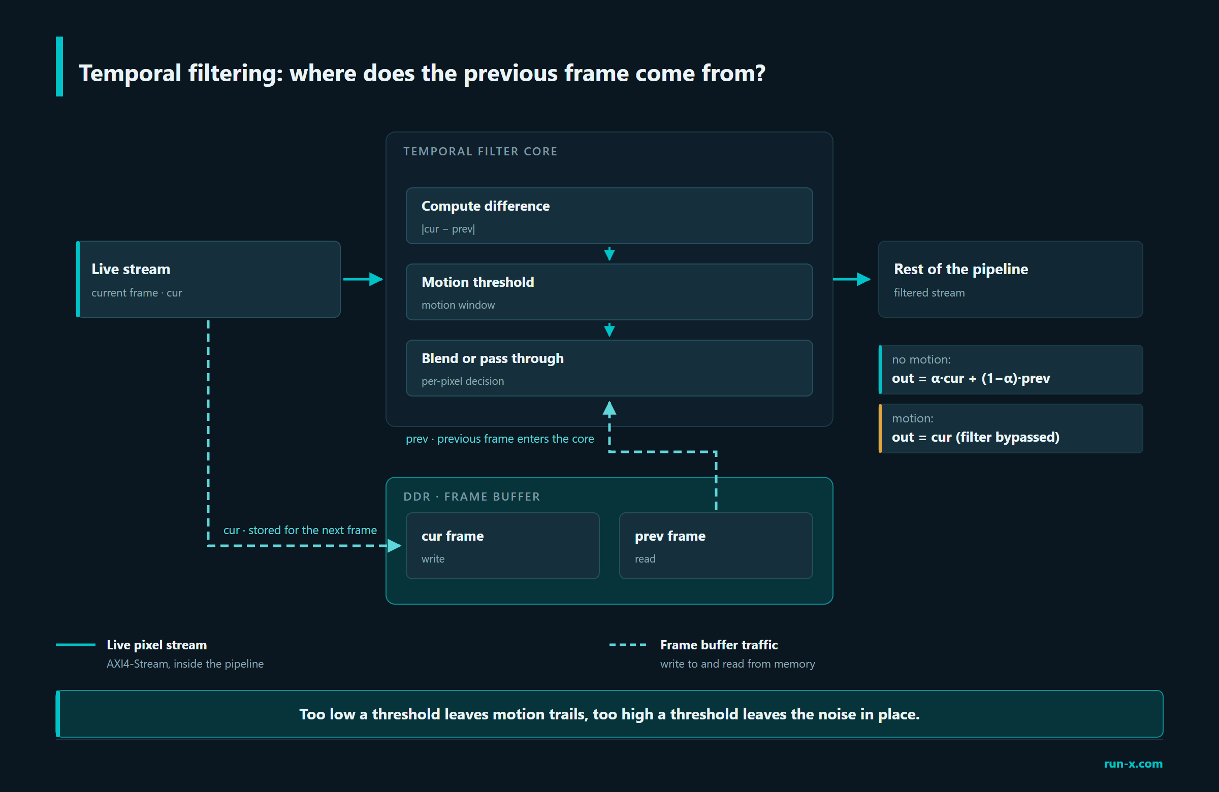
As the live stream moves down the pipeline, a copy of it is written into a frame buffer. On the next frame that copy is read back and handed to the core as a second input. For every pixel the core computes the |cur − prev| difference, compares it against a threshold inside a motion window, and decides: with no motion it blends the two frames, with motion it passes the current frame through untouched.
Where you put the frame buffer matters. This buffer generates constant, regular traffic; if it competes with the rest of the system for the same memory, both it and the other blocks suffer. Where possible, giving it a separate memory region is the cleanest way to add temporal filtering without disturbing anything else.
All of the tuning ends up in the threshold. With no threshold, moving objects leave trails. With too high a threshold the filter barely engages and the noise survives. The right value depends on the scene and the sensor, so it pays to keep the threshold changeable at run time.
The Constraint That Real Time Adds
The real difficulty of building an image processing pipeline on an FPGA is not the algorithms. It is the timing.
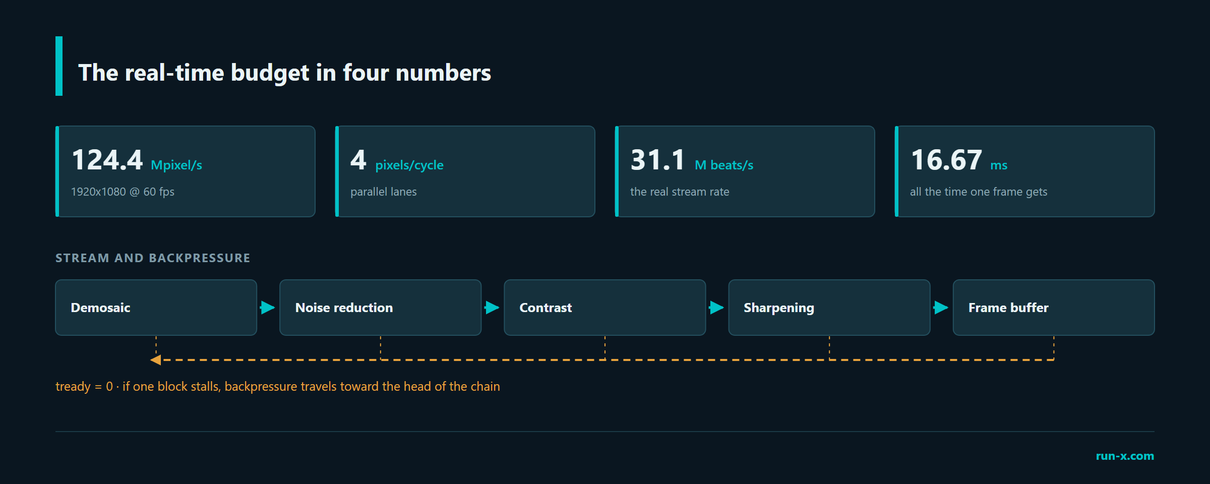
1920x1080 at 60 fps means 124.4 million pixels per second. In a pipeline that handles 4 pixels per clock cycle, that comes to 31.1 million beats per second. The total time you get for one frame is 16.67 ms, and that figure is not open to negotiation.
A streaming pipeline is not a budget, it is a pipe. If a block stalls and does not give the lost cycles back, the FIFO in front of it fills up, tready drops, and backpressure travels toward the head of the chain. That is why fixed latency in every block is a requirement rather than a preference.
What this constraint does to the architecture is a subject of its own: which blocks run with line latency and which force a full frame of delay, where latency accumulates across the system, and how to measure it on hardware. We will cover those in a separate article.
Conclusion
Image processing on an FPGA is not just a matter of translating individual algorithms into hardware. The real work is deciding what order those blocks sit in and how much each of them is allowed to disturb the stream.
The order determines image quality. The noise reduction strategy takes shape according to how the spatial and temporal approaches are combined. And the real-time budget sits above all of it: how well a block performs only counts as long as it never interrupts the flow.
Contact us: info@run-x.com | www.run-x.com