Video Compression and H.264/H.265 Encoding on FPGA
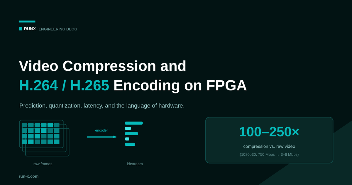
A good video encoder does not compress the picture, it predicts it. The only thing it stores is where its prediction failed.
One second of raw 1080p30 video is about 750 megabits of data. The same video shrinks to between 3 and 8 megabits in H.264, which is a hundred to two hundred and fifty times smaller, and the picture is still perfectly watchable. The encoder does this not by adding anything to the picture, but by throwing away the repetition that is already there. The whole of compression is really hidden in one sentence: the job is not to shrink the data, but to find how much the video repeats itself and to not code that repetition again.
The second point that shapes an FPGA design is this: H.264 is not an algorithm, it is a standard. It fixes only two things, the format of the bitstream and what a decoder will produce from it. It leaves the inside of the encoder completely open. How hard you search for motion, which prediction you choose, how you spread bits across frames, all of that is your decision. So there is no single thing called “an H.264 encoder”; there are countless encoders that obey the same standard, one many times better or many times more expensive than the next. That is also the good news: starting from the simplest version and improving upward, every intermediate step produces a valid video stream that plays and decodes correctly.
In a separate post we described how, in real time image processing, latency depends less on the algorithms and more on which block holds up a single line and which one holds up a whole frame. This post looks at the compression block at the end of that same chain: what is done, why, and how it is done on an FPGA. Let us say it up front, the heart of the matter is mostly not in the math. On hardware, what really sets the cost of a codec is where the data dependencies sit and how the resolution pushes the clock frequency.
Where Compression Happens
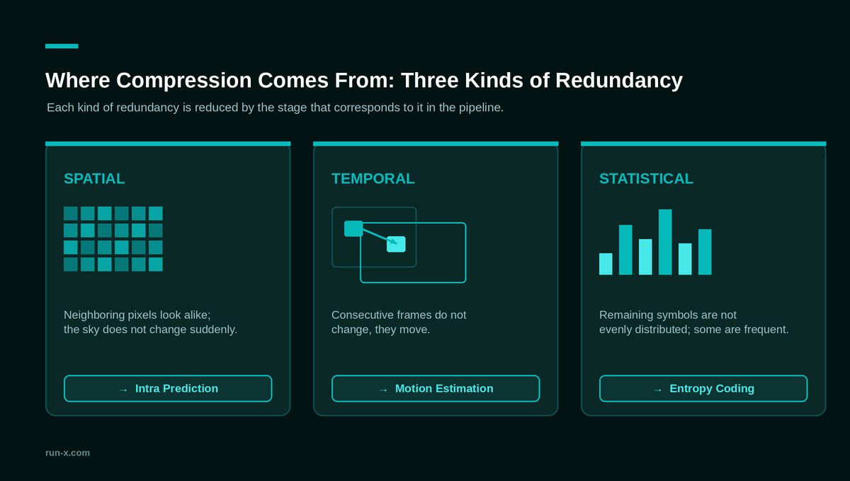
Compression within frames is possible because video data is largely repetitive. The standards target three kinds of this repetition, and each one has a stage that corresponds to it.
- Spatial redundancy. Neighboring pixels in a frame look alike; the sky does not change suddenly. Intra prediction, that is prediction within a frame, reduces this.
- Temporal redundancy. Consecutive frames are almost identical; the content does not change, it moves. Inter prediction, that is motion estimation, reduces this.
- Statistical redundancy. After these steps the remaining symbols are not evenly distributed; some values appear far more often. Entropy coding reduces this.
The logic behind all three is the same. The encoder does not code a block directly; it first predicts it, then codes only how wrong the prediction was, that is the residual. If the prediction is good, the residual is made of small numbers, and small numbers take far less space. The original pixels are never written straight into the bitstream.
The Loss Comes From One Place: Quantization
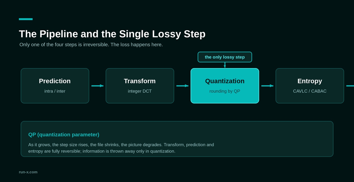
The compression pipeline has four steps: prediction, transform, quantization, entropy. Among these, the only step where information is thrown away is quantization. The transform (an integer DCT in most standards) is lossless and packs the energy into a small number of coefficients. Quantization then divides each coefficient by a step size and rounds it; that operation cannot be undone.
A single number controls the step size: the quantization parameter (QP). As this number grows, the step size grows, more coefficients round to zero and the file gets smaller; in return the picture degrades. So QP is the entire dial between compression and quality.
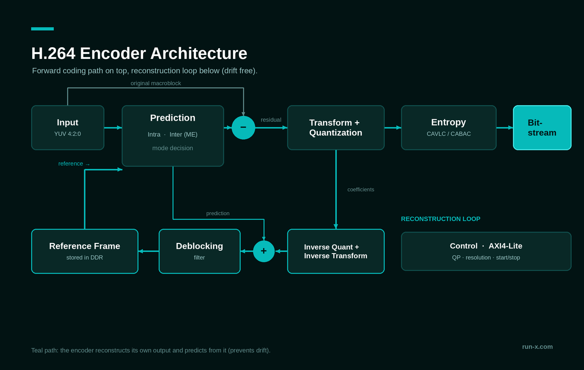
Here is a critical detail that separates a video encoder from a still image compressor. The decoder never sees the original frame, it only holds a somewhat degraded, reconstructed frame. If the encoder predicts future frames from the original frame in its own memory, it relies on data the decoder does not have, and the two drift apart frame by frame. This buildup is called drift; without a single bit going wrong, the picture degrades steadily. The fix is for the encoder to reconstruct its own output exactly as the decoder would, and to predict from that.
This has a concrete consequence on the hardware side. For drift not to occur, the encoder and decoder math must be identical at the bit level. This is why the standards require an integer transform that works only with additions and shifts, instead of a floating point transform. The reason is not speed, it is exactness. The practical meaning is clear: the measure of whether an encoder works correctly is not “does the output look nice”, but “does an independent decoder reconstruct the bitstream bit for bit identically to the frame the encoder produced”.
Why This Work Suits an FPGA
A CPU or a GPU can also do video compression. A few concrete properties set the FPGA apart, and they stand out especially in real time, embedded systems.
The first is predictability. On an FPGA the processing pipeline is a fixed circuit; every frame is processed in the same number of cycles. There is no operating system scheduler, no cache misses, no other processes racing at the same time. In a real time system what matters is not the average speed but the worst case; on an FPGA the worst case and the average are nearly the same.
The second is latency. An FPGA design can start processing line by line, without waiting for the frame to complete. This can push end to end latency below one frame time. In CPU based solutions the frame is first gathered into memory and then processed; that alone adds one frame of latency.
The third is parallelism. As resolution rises, you can scale by building a datapath that processes more than one pixel per cycle. Parallelizing the same work on a single core in software at this scale is hard.
The fourth is power efficiency. Doing the same work in a fixed circuit typically spends far less energy than doing it on a general purpose processor. This becomes decisive at the edge and on mobile platforms, where the power budget is tight.
The fifth is integration. The camera interface, the ISP chain and the compression can sit side by side on the same chip. The image can move from the sensor all the way to being compressed without ever touching external memory or a PCIe link. This reduces both latency and system complexity.
The Cost on Hardware
Most of the compression math is cheap for an FPGA. What is expensive is the serial nature of some of the steps.
There are two common methods in entropy coding. CAVLC is table based; each step is a table lookup and it parallelizes easily on hardware. CABAC is arithmetic coding, it compresses roughly 5 to 15 percent better, but it is serial by construction: coding the next binary decision cannot start until the previous one has finished updating its probability state. This makes no difference in software; in a hardware pipeline it either lowers the throughput or requires a deep, pipelined design. This is why first versions are often built with CAVLC, leaving CABAC to a later stage.
The second cost comes from resolution. A codec’s clock frequency is not found by guessing but by division: you divide the pixel rate by the number of pixels processed per cycle. 1080p30 is about 62 million pixels per second, and 62 MHz is enough for a datapath that processes one pixel per cycle. 1080p60 asks for about 124 MHz, and 4K60 for about 498 MHz. That last figure is above what most FPGA fabric can reach for deep logic like motion estimation. The solution is not to raise the clock but to build a datapath that processes more than one pixel per cycle. But that is not as simple as duplicating the block; neighbor dependent steps like motion search and the deblocking filter resist this widening.
The third cost is memory bandwidth, and this is often the real bottleneck. Motion estimation reads overlapping regions from the reference frame again and again; the reconstructed frame is written back. At high resolution and frame rate this traffic reaches several gigabytes per second on external DDR.
Latency: A Line or a Frame
Every gain in compression is paid for somewhere in latency. The most expensive item is the B-frame. Because a B-frame looks at a frame that comes after it on the timeline, it cannot be shown until that frame has arrived and been decoded. This brings an unavoidable buffering latency; this is why B-frames are mostly not used at all in low latency systems.
I-frames are also a source of latency. An I-frame is far larger than a P-frame, and on a fixed bandwidth channel every I-frame creates a load peak. The common way to fix this is intra refresh: instead of a full I-frame, a few macroblock rows are intra coded in each frame, and a moving band refreshes the whole frame over several frames. This way no large load peak forms and the latency stays constant.
The practical conclusion from this is that shortening the GOP to reduce latency often backfires, because it makes the I-frame peaks more frequent. The right approach is to turn off B-frames, use intra refresh, and build a line based output that starts sending before the frame is complete.
Standards: H.264, H.265 and Beyond
H.264 (AVC) is the most widely used video compression standard today. It is supported by nearly every device, browser and platform, its licensing is settled, and it is a balanced choice for low latency, low power applications. Its drawback is that it spends more bits than newer standards for the same quality.
H.265 (HEVC) is the next generation, and it too is widely used. Its core promise is simple: it delivers the same visual quality at roughly half the bitrate, and this gain becomes especially clear at 4K and 8K. The price is just as heavy. Larger and more flexible block structures, many more prediction modes and mandatory CABAC raise both the compute load and the hardware complexity significantly. Its licensing is also more complex than H.264’s. Later generations (H.266/VVC, AV1) continue this trend: at each step, better compression brings higher complexity.
There is one point worth underlining from the hardware side. Moving from one generation to the next is not a settings change. Moving to H.265 means redesigning almost every block, from the block structure to the entropy coder; the only thing that carries over is not the RTL but the design and verification methodology. For this reason the common path in practice is to build a solid and portable base with H.264, and to plan later generations as separate projects.
There is one more point of comparison. On some devices the video codec is already embedded as a fixed, hard block. The value of soft IP is not to compete with it on cost, but to meet a different need: portability across FPGA vendors, customizability, and very low latency. Being able to run a single RTL on the fabric of more than one vendor makes soft IP valuable where the hard block cannot reach.
In the end, video compression is not a speed race. It is the work of turning the predictability of video into bits, and bits into a latency and memory budget. The loss gathers in one place, in quantization. The hardware cost gathers not in the math, but in the serial dependencies and in the pressure that resolution puts on the clock.
The FPGA is a strong option in this equation: fixed and predictable latency, line level processing, parallelism that scales with resolution, and integration close to the sensor. These properties become decisive especially in real time and embedded imaging systems.
At RunX we develop vendor independent video compression solutions that run on FPGA. You can contact the RunX engineering team for your video compression solutions.
Get in Touch: info@run-x.com | www.run-x.com