Radar Signal Processing on FPGA

From raw echoes to detections: why the processing chain is the real radar, and why FPGAs sit at its core.
A radar antenna does not deliver targets. It delivers voltages: a faint echo buried in noise, clutter and interference, sampled billions of times a second. Everything we call “radar performance” (how far it sees, how small a target it resolves, how fast an object it can measure, how quickly it reacts) is decided after the ADC, in the signal processing chain.
That is why radar design is, to a large extent, a processing architecture problem. In this article we walk through what a radar has to compute, using pulse-Doppler as a worked example, why that workload is so demanding, why FPGAs are the natural fit for it, and what a practical antenna → AFE → FPGA architecture looks like.
Why radar needs signal processing
Radar echoes are extremely weak, and they get weaker fast: the power returning from a target falls with the fourth power of its distance. In the same receive window, a nearby strong reflector (ground clutter, a building, a large vehicle) and a distant small target can differ in level by 100 dB or more. The receiver has to represent both at once, then separate them.
The goal of processing is to turn that raw stream into three physical quantities for every target: range (how far), velocity (how fast, and in which direction) and, with an antenna array, angle. None of these is directly measured. Each is extracted by transforming and filtering the sampled signal.
Radar processing chains: a pulse-Doppler example
There is no single radar processing algorithm; the chain depends on the waveform and the application. FMCW radars, common in automotive and industrial sensing, transmit continuous chirps and recover range with an FFT across the samples of each chirp, velocity with a second FFT across consecutive chirps, and angle with a third across the antenna elements, which together form the so-called radar data cube. Array radars add beamforming on top, and pulsed systems rely on pulse compression and Doppler filtering.
The details differ, but the structure is shared: digitize, condition, transform along fast time, slow time and, for arrays, the spatial dimension, then detect. To make that structure concrete, we follow a pulse-Doppler radar, where each stage is easy to see on its own. Many of the same building blocks (FFTs, filtering and adaptive detection) reappear in other radar types.
A pulse-Doppler radar transmits a train of pulses and processes the returns across two time scales: within each pulse (fast time, which carries range) and from pulse to pulse (slow time, which carries Doppler). A typical chain looks like this.
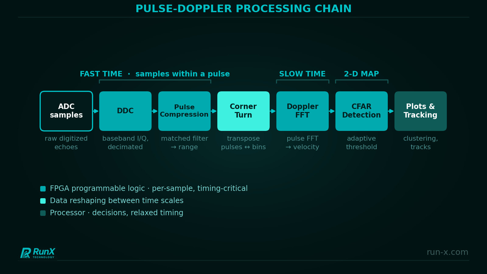
Digital down-conversion (DDC): The ADC output is shifted to baseband, filtered and decimated into I/Q samples. This reduces the data rate to what the rest of the chain actually needs and is the first stage that sees the full sample stream.
Pulse compression: To get long-range detection without needing enormous peak power, the radar transmits a long, modulated pulse (for example a chirp) and compresses it in the receiver with a matched filter: the echo is correlated against a replica of the transmitted waveform, and a sharp peak appears where the target is. Range resolution is set by the bandwidth, ΔR = c / 2B. A 20 µs pulse spanning 10 MHz resolves roughly 15 m in range. An uncompressed pulse would need to be about 100 ns long to match that, and would carry a fraction of the energy. Short filters (up to a few thousand samples) are typically implemented as time-domain FIR filters. Long chirps are usually handled in the frequency domain, with FFT, multiplication and inverse FFT.
Corner turn: The data arrives pulse by pulse, but Doppler processing needs it across pulses for each range bin. The data matrix has to be transposed, a “corner turn”, and this step demands very low-latency memory access, from either large on-chip memory or fast external RAM.
Doppler FFT: For every range bin, an FFT across the pulses separates targets by velocity and pushes stationary clutter into a known, rejectable region of the spectrum. Windowing is applied first to control spectral leakage.
Detection (CFAR): The result is a range-Doppler map. A Constant False Alarm Rate (CFAR) detector compares each cell against a threshold adapted to its surrounding noise and clutter level, so the false-alarm rate stays stable as conditions change.
Plot extraction and tracking: Detections are clustered into plots, associated over time into tracks, and delivered to the application. This is decision-making work with relaxed timing, and it sits naturally on a processor.
Why this workload is hard
The first difficulty is sheer rate. Wideband radars sample at very high rates, and array radars multiply that by every channel; AESA radars can have hundreds or even thousands of separate receive/transmit units. The second is dimensionality: processing happens in two dimensions at once, time for pulse compression and frequency for Doppler, so the data has to be reshaped in the middle of the chain. The third is numeric: the dynamic range described earlier has to survive every stage, so word lengths and scaling are architectural decisions, not afterthoughts.
Finally, the whole thing is real-time. A radar that processes a coherent interval slower than it collects it falls behind forever, and extra latency directly delays the system’s reaction.
Algorithms help (a 1024-point FFT needs only about 1% of the arithmetic of a direct DFT), but the efficient algorithm is only half the story. The other half is a hardware architecture that can feed it continuously.
Why FPGAs
Deterministic, low latency. An FPGA pipeline processes samples as they arrive, with fixed, known latency, independent of operating-system scheduling, caches or interrupts. For processing close to the sensor this is the decisive property.
Parallelism that matches the problem. Hardware resources can be arranged and interconnected in parallel to meet even demanding real-time requirements: many channels, many beams, many range bins at once. Adding channels means adding logic, not slowing down what is already running.
Direct access to wideband converters. FPGAs provide configurable high-speed interfaces to wideband ADCs and DACs at gigahertz sampling rates, along with memory controllers fast enough to feed the corner turn. The sample stream enters the processing logic without an intermediate bus or driver layer.
Efficiency and reconfigurability. With thousands of DSP blocks available, FPGAs deliver a lot of processing per watt, which matters in embedded and mobile platforms. And because the logic is reprogrammable, waveforms, filters and detection schemes can be updated in the field, something a fixed ASIC cannot offer.
FPGAs and processors, better together
Not every stage of a radar needs nanosecond determinism. Tracking, scheduling, display and networking are decision-making tasks with relaxed timing, and they are best served by a processor. This is exactly what FPGA SoC platforms are built for: a processing system (PS) with ARM cores and the programmable logic (PL) sit on the same silicon, with a high-bandwidth data path between them. The per-sample signal chain runs in the PL, while the PS takes on the work that software does best. That is why modern radar systems usually split the work, and why SoC designs are such a natural fit for them. Our rule of thumb is simple: if a job needs a timing guarantee or runs per sample, it belongs in the programmable logic; if it makes decisions or talks to the outside world, it belongs on the PS. The result is a system that is deterministic where it has to be and flexible everywhere else.
A reference architecture: antenna → AFE → FPGA
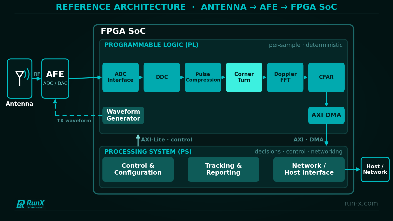
The block diagram above shows a generic arrangement; real systems vary with the radar type, the converter and the platform.
The antenna and RF front end shape and condition the signal: filtering, amplification and frequency conversion. The analog front end (AFE) digitizes the received signal with an ADC, and on the transmit side a DAC generates the waveform. Between the AFE and the FPGA, high-speed serial links (JESD204 is common) carry samples, so interface bring-up and clocking are real design work, not plumbing.
Inside the FPGA’s programmable logic (PL), the per-sample, timing-critical chain runs: the serial interface receiver, DDC, pulse compression, corner-turn buffering, Doppler FFT and CFAR. Streaming interfaces connect these stages so that data flows through without stalling, and DMA moves results into memory with minimal processor involvement.
The processing system (PS) on an FPGA SoC handles what a processor does best: configuring the PL blocks, tracking and reporting, network communication, system management and updates. If you want the details of how we divide work between PS and PL, the AXI interfaces we use, and why DMA matters, we’ve covered that in a separate article, linked below.
Design decisions that matter
A few choices tend to determine whether a radar processing design succeeds. Fixed-point word lengths and scaling must preserve the dynamic range without wasting DSP resources. The corner turn must be sized and scheduled so that memory bandwidth never becomes the bottleneck. Clocking and the converter interface must be validated early, because they gate everything downstream. Verification must run with realistic data, not only with unit tests. And the balance between hand-written RTL and high-level synthesis should be decided per block, based on timing criticality and reuse.
Continue the Series
If you want to go deeper on how the PS and PL cooperate in a radar-class data path, read PS/PL Architecture in FPGA SoC Devices. Also radar data and camera frames share a lot in common: both are 2D arrays processed as streams. For a deeper look at 2D image signal processing on FPGAs, see Image Signal Processing on FPGAs: Pipelines and Noise Reduction.
If you are working on a radar or other high-rate sensing system and want to talk through the signal processing architecture, we’d love to hear from you.
Talk to us: info@run-x.com | [www.run-x.com](https://www.run-x.com)